5 Multi-Conc Results Analysis

5.1 Import MC data

#Get the spid of the 169 chemicals entering multi-con test.
dt_mc_ls <- read_csv("./input data files/NIS_ph1_v2_mc_lvl0_for_tcpl_raiu.csv", na = "NA") %>% select(spid)
mc_chem_list <- unique(dt_mc_ls$spid)[-(1:6)]
ls169 <- sc_median %>%
    filter(mc_test=="Yes") %>%
    dplyr::select(spid)

ls11 <- data.frame(mc_chem_list) %>%
    mutate(flag = (mc_chem_list %in% ls169$spid)) %>%
    filter(flag==FALSE) %>%
    dplyr::select(mc_chem_list) %>% rename(spid=mc_chem_list)

spid_chnm_table <- read_excel("./raw data files/EPA_11700_EPA-SLaws_ph1v2_150ul_20170125_key.xlsx")

spid_chnm_table <- spid_chnm_table %>% dplyr::select(EPA_Sample_ID, CASRN, Preferred_Name)
# rename the column title to be compatible with tcpl package. 
names(spid_chnm_table) <- c("spid", "casn", "chnm")

# Import MC data (look at the 169 chemicals)
mc_lvl0_raiu_update <- 
    read_csv("./input data files/NIS_ph1_v2_mc_lvl0_for_tcpl_raiu.csv") %>%
    filter(!(spid %in% ls11$spid))

mc_lvl0_cyto_update <- 
    read_csv("./input data files/NIS_ph1_v2_mc_lvl0_for_tcpl_cytotox.csv") %>% 
    filter(!(spid %in% ls11$spid))

dt_mc <- bind_rows(mc_lvl0_cyto_update, mc_lvl0_raiu_update)

5.2 Normalization

Normalize raw response to the median of DMSO controls, calculated per plate.

dt_mc_norm <- toxplot::normalize_per_plate(dt_mc)

5.3 3bMAD of MC

#create concentration index
dt_mc_norm <- dt_mc_norm %>% 
    group_by(spid) %>% 
    mutate(cndx = generate_index(conc)) %>% 
    ungroup
sig_mc <- dt_mc_norm %>% 
  mutate(neg_nval_median= 100 - nval_median) %>% 
  group_by(assay) %>% 
  dplyr::filter(wllt == "t") %>% 
  dplyr::filter(cndx == 1 | cndx == 2) %>%    
  summarise(bMAD = mad(neg_nval_median, na.rm = TRUE),
            three_bMAD=3*mad(neg_nval_median, na.rm = TRUE)) 
knitr::kable(sig_mc, digits =2)

assay	bMAD	three_bMAD
Cytotox	5.89	17.68
RAIU	7.93	23.78

5.4 Multi-Con QC

5.4.1 Quality Control

To assesss the quality of assay for each 96 well plate, the following metrics were used .

* CV of DMSO controls 
* Z' score

The negative control DMSO wells’ raw readings were used to calculate mean, standard deviation and CV for each plate.
Z’ score and SSMD were calculated for each plate as well using the raw data of DMSO negative control, RAIU or cytotox positive control readings. Note the positive control values are taken from the highest concentration wells, which represent the maximum RAIU inhibition or toxic inhibition observed on the positive control chemicals.

Z’ factor is calculated as follows:
\[Z'=1-\frac{3\sigma_{positive\ control} + 3\sigma_{DMSO\ control}}{|\mu_{positive\ control} - \mu_{DMSO\ control}|}\]

**Note that in Z’ calculation, because we only had one well of cytotox positive control, therefore sigma wasn’t calculatable. This make the cytotox Z’ score looks better than the RAIU.

# function to calculate CV_DMSO, Z' and SSMD for each plate
# Note the calculation is based on raw/unnormalized data. 
#dt_mc_norm <- readRDS("dt_mc_norm.rds")

qc_mc <- qc_per_plate(dt_mc_norm, assay_info, resp = "nval_median")
#qc_l <- qc %>% gather(metric, value, CV_DMSO:SSMD) 

# qplot(unique_id, SSMD, data=qc, color = assay_name) + theme(axis.text.x=element_blank(), axis.ticks.x=element_blank())
qplot(unique_id, CV_DMSO, data=qc_mc$qc, color = assay) + 
    ggtitle("CV of DMSO in Multi-Con Assay") +
    xlab("Assay Plate ID")+
    scale_x_discrete(labels=NULL)+
    theme_bw()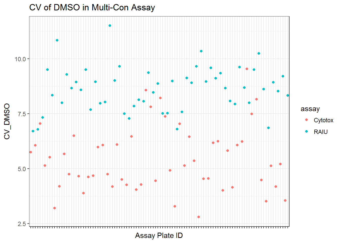

    #theme(axis.text.x=element_blank(),axis.ticks.x=element_blank())

qplot(unique_id, Z_prime, data=qc_mc$qc, color = assay) + 
    ggtitle("Z' Score in Multi-Con Assay") + 
    xlab("Assay Plate ID")+
    scale_x_discrete(labels=NULL) + 
    theme_bw()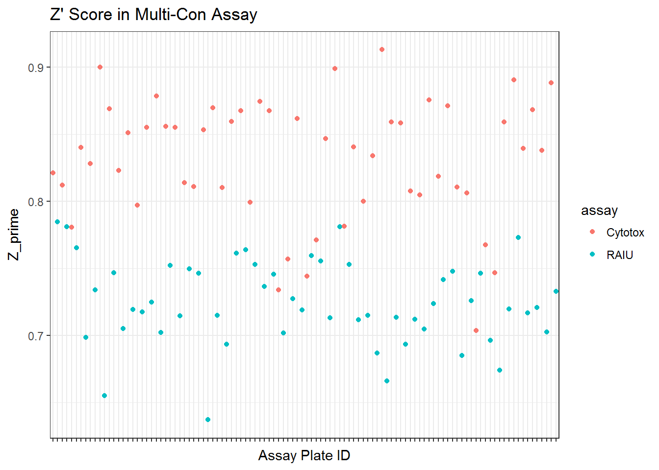

    #theme(axis.text.x=element_blank(),axis.ticks.x=element_blank())

The summary of qulaity control metrics for Multi-conc Cell Viability Assay:

qc_mc_cyto <- qc_mc$qc %>% filter(assay == "Cytotox") %>%  
    dplyr::select(CV_DMSO, Z_prime) %>%
    describe
knitr::kable(qc_mc_cyto[2:3,], digits = 2, 
             caption = "Summary of Multi-Conc Cell Viability Assay QC Metrics")

Table 5.1: Summary of Multi-Conc Cell Viability Assay QC Metrics
	vars	n	mean	sd	median	trimmed	mad	min	max	range	skew	kurtosis	se
CV_DMSO	2	54	5.42	1.47	5.14	5.32	1.40	2.8	9.54	6.74	0.64	-0.09	0.20
Z_prime	3	54	0.83	0.05	0.84	0.83	0.04	0.7	0.91	0.21	-0.63	-0.10	0.01

Summary of qc metrics for Multi-conc RAIU assay:

qc_mc_r <- qc_mc$qc %>% filter(assay == "RAIU") %>%  
    dplyr::select(CV_DMSO, Z_prime) %>%
    describe

## Adding missing grouping variables: `apid`

## Warning: NAs introduced by coercion

## Warning in FUN(newX[, i], ...): no non-missing arguments to min; returning
## Inf

## Warning in FUN(newX[, i], ...): no non-missing arguments to max; returning
## -Inf

knitr::kable(qc_mc_r[2:3,], caption="Summary Multi-Conc RAIU Assay QC Metrics")

Table 5.2: Summary Multi-Conc RAIU Assay QC Metrics
	vars	n	mean	sd	median	trimmed	mad	min	max	range	skew	kurtosis	se
CV_DMSO	2	54	8.6167424	1.014914	8.6613033	8.598188	1.0016105	6.704893	11.4977674	4.7928743	0.2629207	0.0569357	0.1381124
Z_prime	3	54	0.7244648	0.031661	0.7202322	0.725418	0.0337723	0.637237	0.7846036	0.1473666	-0.2947822	-0.0649648	0.0043085

All qc metrics in a table:

knitr::kable(dplyr::select(qc_mc$qc, apid, assay, CV_DMSO, Z_prime),
             digits = 2,
             longtable = TRUE,
             col.names = c("Plate", "assay","CV of DMSO", "Z'"),
             caption = "Plate-wise quality control metrics in Multi-Conc Assays")

(#tab:qc table)Plate-wise quality control metrics in Multi-Conc Assays
Plate	assay	CV of DMSO	Z’
Plate_1_rep1	RAIU	6.70	0.78
Plate_1_rep2	RAIU	6.78	0.78
Plate_1_rep3	RAIU	7.33	0.77
Plate_10_rep1	RAIU	9.50	0.70
Plate_10_rep2	RAIU	8.34	0.73
Plate_10_rep3	RAIU	10.84	0.66
Plate_11_rep1	RAIU	8.00	0.75
Plate_11_rep2	RAIU	9.28	0.70
Plate_11_rep3	RAIU	8.66	0.72
Plate_12_rep1	RAIU	8.93	0.72
Plate_12_rep2	RAIU	8.59	0.72
Plate_12_rep3	RAIU	9.50	0.70
Plate_13_rep1	RAIU	7.68	0.75
Plate_13_rep2	RAIU	8.95	0.71
Plate_13_rep3	RAIU	7.97	0.75
Plate_14_rep1	RAIU	8.02	0.75
Plate_14_rep2	RAIU	11.50	0.64
Plate_14_rep3	RAIU	9.01	0.71
Plate_15_rep1	RAIU	9.65	0.69
Plate_15_rep2	RAIU	7.50	0.76
Plate_15_rep3	RAIU	7.28	0.76
Plate_16_rep1	RAIU	7.85	0.75
Plate_16_rep2	RAIU	8.13	0.74
Plate_16_rep3	RAIU	8.06	0.75
Plate_17_rep1	RAIU	9.37	0.70
Plate_17_rep2	RAIU	8.46	0.73
Plate_17_rep3	RAIU	8.87	0.72
Plate_18_rep1	RAIU	7.51	0.76
Plate_18_rep2	RAIU	7.52	0.76
Plate_18_rep3	RAIU	8.98	0.71
Plate_2_rep1	RAIU	6.80	0.78
Plate_2_rep2	RAIU	7.58	0.75
Plate_2_rep3	RAIU	9.12	0.71
Plate_3_rep1	RAIU	8.90	0.72
Plate_3_rep2	RAIU	9.66	0.69
Plate_3_rep3	RAIU	10.34	0.67
Plate_4_rep1	RAIU	8.96	0.71
Plate_4_rep2	RAIU	9.59	0.69
Plate_4_rep3	RAIU	9.11	0.71
Plate_5_rep1	RAIU	9.34	0.70
Plate_5_rep2	RAIU	8.66	0.72
Plate_5_rep3	RAIU	8.07	0.74
Plate_6_rep1	RAIU	7.94	0.75
Plate_6_rep2	RAIU	9.61	0.69
Plate_6_rep3	RAIU	8.69	0.73
Plate_7_rep1	RAIU	7.99	0.75
Plate_7_rep2	RAIU	9.49	0.70
Plate_7_rep3	RAIU	10.23	0.67
Plate_8_rep1	RAIU	8.61	0.72
Plate_8_rep2	RAIU	6.85	0.77
Plate_8_rep3	RAIU	8.93	0.72
Plate_9_rep1	RAIU	8.52	0.72
Plate_9_rep2	RAIU	9.20	0.70
Plate_9_rep3	RAIU	8.33	0.73
Plate_1_rep1	Cytotox	5.75	0.82
Plate_1_rep2	Cytotox	6.06	0.81
Plate_1_rep3	Cytotox	7.05	0.78
Plate_10_rep1	Cytotox	5.14	0.84
Plate_10_rep2	Cytotox	5.52	0.83
Plate_10_rep3	Cytotox	3.21	0.90
Plate_11_rep1	Cytotox	4.19	0.87
Plate_11_rep2	Cytotox	5.67	0.82
Plate_11_rep3	Cytotox	4.75	0.85
Plate_12_rep1	Cytotox	6.50	0.80
Plate_12_rep2	Cytotox	4.66	0.86
Plate_12_rep3	Cytotox	3.89	0.88
Plate_13_rep1	Cytotox	4.62	0.86
Plate_13_rep2	Cytotox	4.68	0.85
Plate_13_rep3	Cytotox	5.98	0.81
Plate_14_rep1	Cytotox	6.08	0.81
Plate_14_rep2	Cytotox	4.74	0.85
Plate_14_rep3	Cytotox	4.19	0.87
Plate_15_rep1	Cytotox	6.10	0.81
Plate_15_rep2	Cytotox	4.50	0.86
Plate_15_rep3	Cytotox	4.27	0.87
Plate_16_rep1	Cytotox	6.46	0.80
Plate_16_rep2	Cytotox	4.05	0.87
Plate_16_rep3	Cytotox	4.28	0.87
Plate_17_rep1	Cytotox	8.56	0.73
Plate_17_rep2	Cytotox	7.81	0.76
Plate_17_rep3	Cytotox	4.45	0.86
Plate_18_rep1	Cytotox	8.21	0.74
Plate_18_rep2	Cytotox	7.37	0.77
Plate_18_rep3	Cytotox	4.92	0.85
Plate_2_rep1	Cytotox	3.29	0.90
Plate_2_rep2	Cytotox	7.04	0.78
Plate_2_rep3	Cytotox	5.14	0.84
Plate_3_rep1	Cytotox	6.45	0.80
Plate_3_rep2	Cytotox	5.35	0.83
Plate_3_rep3	Cytotox	2.80	0.91
Plate_4_rep1	Cytotox	4.54	0.86
Plate_4_rep2	Cytotox	4.55	0.86
Plate_4_rep3	Cytotox	6.17	0.81
Plate_5_rep1	Cytotox	6.25	0.80
Plate_5_rep2	Cytotox	4.01	0.88
Plate_5_rep3	Cytotox	5.82	0.82
Plate_6_rep1	Cytotox	4.15	0.87
Plate_6_rep2	Cytotox	6.07	0.81
Plate_6_rep3	Cytotox	6.23	0.81
Plate_7_rep1	Cytotox	9.54	0.70
Plate_7_rep2	Cytotox	7.48	0.77
Plate_7_rep3	Cytotox	8.16	0.75
Plate_8_rep1	Cytotox	4.48	0.86
Plate_8_rep2	Cytotox	3.52	0.89
Plate_8_rep3	Cytotox	5.13	0.84
Plate_9_rep1	Cytotox	4.19	0.87
Plate_9_rep2	Cytotox	5.21	0.84
Plate_9_rep3	Cytotox	3.56	0.89

5.4.2 Sodium Perchlorate & DCNQ

On each assay plate, sodium perchlorate and DCNQ were included in six concentrations to serve as positive controls for RAIU and Cytotox assay. Here they are modelled separately by each assay plate.

##extract mc related data frame
d_pos_cyto <- dt_mc_norm %>% filter(assay == "Cytotox", wllt== "pc")
d_pos_raiu <- dt_mc_norm %>% filter(assay == "RAIU", wllt=="pr")

d_neg_cyto <- dt_mc_norm %>% filter(assay == "Cytotox", wllt=="nrc")
d_neg_raiu <- dt_mc_norm %>% filter(assay == "RAIU", wllt=="nrc")
d_ec80_raiu <- dt_mc_norm %>% filter(assay == "RAIU", wllt=="pr_ec80")
d_ec20_raiu <- dt_mc_norm %>% filter(assay == "RAIU", wllt=="pr_ec20")

##plot all DCNQ in multi-con
g_cyto_pos <- qplot(data=d_pos_cyto, x=log10(conc), y=nval_median) +
    labs(
        #title = paste("SPID: " , spid, "\nNAME: ", chnm, "\nCAS NO: ", casn, sep = ""),
        x = "Concentration (logM)",
        y = "% Control Activity"
    ) +
    geom_point(
        color = "#F8766D",
        shape = 1,
        alpha = 0.5,
        size = 1.8
    ) +
    coord_fixed(
        ylim = c(0, 125),
        xlim = c(-9, -4),
        ratio = 2 / 70
    ) +
    scale_y_continuous(breaks = seq(
        from = 0,
        to = 120,
        by = 20
    )) +
    theme_bw() +
    # scale_color_manual(values=c("red","blue"))+
    theme(legend.title = element_blank())+
    theme(plot.title=element_text(hjust=0.5))
g_cyto_pos

##plot all NaClO4 in multi-con
g_raiu_pos <- qplot(data=d_pos_raiu, x=log10(conc), y=nval_median) +
    labs(
        #title = paste("SPID: " , spid, "\nNAME: ", chnm, "\nCAS NO: ", casn, sep = ""),
        x = "Concentration (logM)",
        y = "% Control Activity"
    ) +
    geom_point(
        color = "#00BFC4",
        shape = 1,
        alpha = 0.5,
        size = 1
    ) +
    coord_fixed(
        ylim = c(0, 125),
        xlim = c(-9, -4),
        ratio = 2 / 70
    ) +
    scale_y_continuous(breaks = seq(
        from = 0,
        to = 120,
        by = 20
    )) +
    theme_bw() +
    theme(legend.title = element_blank())+
    theme(plot.title=element_text(hjust=0.5))

g_raiu_pos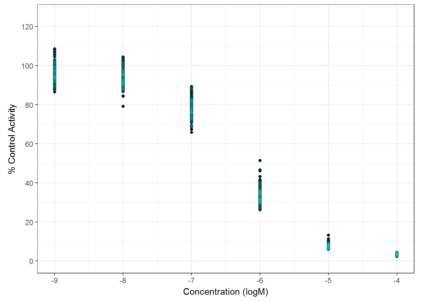

# Obtain AC50 and absEC50 for the positive controls

d_pos_raiu <- mutate(d_pos_raiu, spid = paste(spid, apid, sep = "_"))
pos_raiu_md <- toxplot::fit_curve_tcpl(df = d_pos_raiu,
                                 assay_info = list(prim_assay = "RAIU", toxi_assay = NULL))

## Processing 54 samples(spid)....
## NaClO4_Plate_1_rep1 ||NaClO4_Plate_1_rep2 ||NaClO4_Plate_1_rep3 ||NaClO4_Plate_10_rep1 ||NaClO4_Plate_10_rep2 ||NaClO4_Plate_10_rep3 ||NaClO4_Plate_11_rep1 ||NaClO4_Plate_11_rep2 ||NaClO4_Plate_11_rep3 ||NaClO4_Plate_12_rep1 ||NaClO4_Plate_12_rep2 ||NaClO4_Plate_12_rep3 ||NaClO4_Plate_13_rep1 ||NaClO4_Plate_13_rep2 ||NaClO4_Plate_13_rep3 ||NaClO4_Plate_14_rep1 ||NaClO4_Plate_14_rep2 ||NaClO4_Plate_14_rep3 ||NaClO4_Plate_15_rep1 ||NaClO4_Plate_15_rep2 ||NaClO4_Plate_15_rep3 ||NaClO4_Plate_16_rep1 ||NaClO4_Plate_16_rep2 ||NaClO4_Plate_16_rep3 ||NaClO4_Plate_17_rep1 ||NaClO4_Plate_17_rep2 ||NaClO4_Plate_17_rep3 ||NaClO4_Plate_18_rep1 ||NaClO4_Plate_18_rep2 ||NaClO4_Plate_18_rep3 ||NaClO4_Plate_2_rep1 ||NaClO4_Plate_2_rep2 ||NaClO4_Plate_2_rep3 ||NaClO4_Plate_3_rep1 ||NaClO4_Plate_3_rep2 ||NaClO4_Plate_3_rep3 ||NaClO4_Plate_4_rep1 ||NaClO4_Plate_4_rep2 ||NaClO4_Plate_4_rep3 ||NaClO4_Plate_5_rep1 ||NaClO4_Plate_5_rep2 ||NaClO4_Plate_5_rep3 ||NaClO4_Plate_6_rep1 ||NaClO4_Plate_6_rep2 ||NaClO4_Plate_6_rep3 ||NaClO4_Plate_7_rep1 ||NaClO4_Plate_7_rep2 ||NaClO4_Plate_7_rep3 ||NaClO4_Plate_8_rep1 ||NaClO4_Plate_8_rep2 ||NaClO4_Plate_8_rep3 ||NaClO4_Plate_9_rep1 ||NaClO4_Plate_9_rep2 ||NaClO4_Plate_9_rep3 ||
## Curve Fitting Completed!
## Calculation time: 9.1 secs

raiu_pos_tbl <- toxplot::summary_tcpl(pos_raiu_md)


d_pos_cyto <- mutate(d_pos_cyto, spid = paste(spid, apid, sep = "_"))
pos_cyto_md <- toxplot::fit_curve_tcpl(df = d_pos_cyto,
                                 assay_info = list(prim_assay = NULL, toxi_assay = "Cytotox"))

## Processing 54 samples(spid)....
## DCNQ_Plate_1_rep1 ||DCNQ_Plate_1_rep2 ||DCNQ_Plate_1_rep3 ||DCNQ_Plate_10_rep1 ||DCNQ_Plate_10_rep2 ||DCNQ_Plate_10_rep3 ||DCNQ_Plate_11_rep1 ||DCNQ_Plate_11_rep2 ||DCNQ_Plate_11_rep3 ||DCNQ_Plate_12_rep1 ||DCNQ_Plate_12_rep2 ||DCNQ_Plate_12_rep3 ||DCNQ_Plate_13_rep1 ||DCNQ_Plate_13_rep2 ||DCNQ_Plate_13_rep3 ||DCNQ_Plate_14_rep1 ||DCNQ_Plate_14_rep2 ||DCNQ_Plate_14_rep3 ||DCNQ_Plate_15_rep1 ||DCNQ_Plate_15_rep2 ||DCNQ_Plate_15_rep3 ||DCNQ_Plate_16_rep1 ||DCNQ_Plate_16_rep2 ||DCNQ_Plate_16_rep3 ||DCNQ_Plate_17_rep1 ||DCNQ_Plate_17_rep2 ||DCNQ_Plate_17_rep3 ||DCNQ_Plate_18_rep1 ||DCNQ_Plate_18_rep2 ||DCNQ_Plate_18_rep3 ||DCNQ_Plate_2_rep1 ||DCNQ_Plate_2_rep2 ||DCNQ_Plate_2_rep3 ||DCNQ_Plate_3_rep1 ||DCNQ_Plate_3_rep2 ||DCNQ_Plate_3_rep3 ||DCNQ_Plate_4_rep1 ||DCNQ_Plate_4_rep2 ||DCNQ_Plate_4_rep3 ||DCNQ_Plate_5_rep1 ||DCNQ_Plate_5_rep2 ||DCNQ_Plate_5_rep3 ||DCNQ_Plate_6_rep1 ||DCNQ_Plate_6_rep2 ||DCNQ_Plate_6_rep3 ||DCNQ_Plate_7_rep1 ||DCNQ_Plate_7_rep2 ||DCNQ_Plate_7_rep3 ||DCNQ_Plate_8_rep1 ||DCNQ_Plate_8_rep2 ||DCNQ_Plate_8_rep3 ||DCNQ_Plate_9_rep1 ||DCNQ_Plate_9_rep2 ||DCNQ_Plate_9_rep3 ||
## Curve Fitting Completed!
## Calculation time: 5.4 secs

cyto_pos_tbl <- toxplot::summary_tcpl(pos_cyto_md) 

pos_tbl <- bind_rows(cyto_pos_tbl, raiu_pos_tbl)  #this is the modelling results for all mc positive

5.4.2.1 Visualize AC50s

ggplot(raiu_pos_tbl, aes(spid, AC50_prim)) +
    geom_point(alpha=0.8, size=3)+
    scale_x_discrete(labels=NULL)+
    ggtitle("AC50 of RAIU Positive Control (NaClO4) in Multi-Conc Assay")+
    xlab("Assay Plate ID") +
    ylab("Concentration (logM)") +
    theme(plot.title = element_text(hjust=0.5)) +
    theme_bw()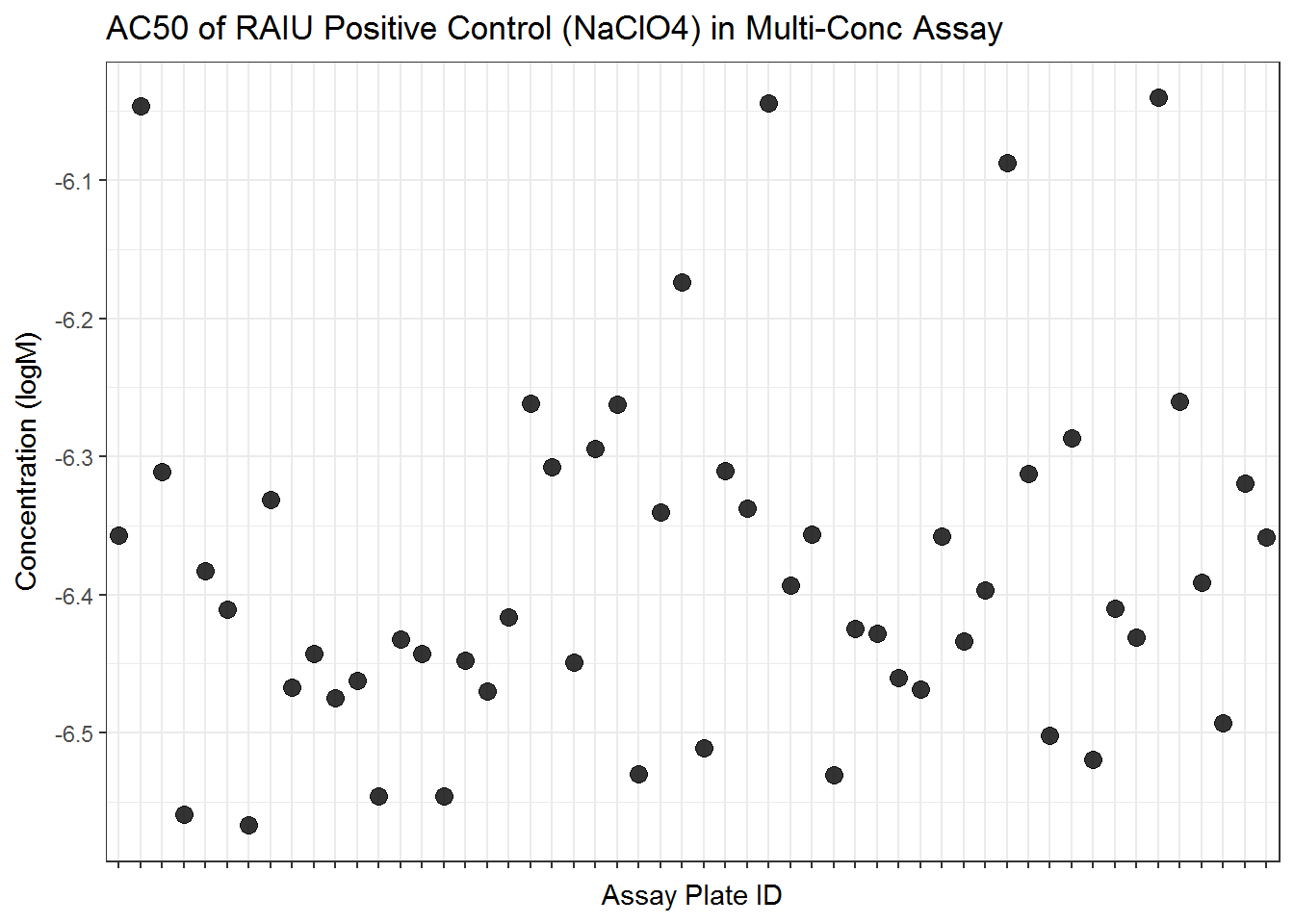

ggplot(cyto_pos_tbl, aes(spid, AC50_toxi)) +
    geom_point(alpha=0.8, size=3)+
    #facet_grid(Metric~., scale="free")+
    scale_x_discrete(labels=NULL)+
    ggtitle("AC50 of Cell Viability Positive Control (DCNQ) in Multi-Conc Assay")+
    xlab("Assay Plate ID") +
    ylab("Concentration (logM)") +
    theme(plot.title = element_text(hjust=0.5)) +
    theme_bw()

5.4.2.2 Summarize AC50s of positive controls in multi-conc assays

##summarizing AC50s of positive controls.
library(psych)
pos_sum_raiu <- raiu_pos_tbl %>%
    dplyr::select(AC50_prim, absEC50_prim) %>% 
    describe

pos_sum_cyto <- cyto_pos_tbl %>%
    dplyr::select(AC50_toxi, absEC50_toxi) %>% 
    describe

knitr::kable(pos_sum_raiu, digits = 2,  caption="Summary of RAIU positive control IC50s")

Table 5.3: Summary of RAIU positive control IC50s
	vars	n	mean	sd	median	trimmed	mad	min	max	range	skew	kurtosis	se
AC50_prim	1	54	-6.38	0.13	-6.41	-6.40	0.11	-6.57	-6.04	0.53	1.04	0.83	0.02
absEC50_prim	2	54	-6.36	0.13	-6.39	-6.38	0.10	-6.54	-6.04	0.51	0.89	0.52	0.02

knitr::kable(pos_sum_cyto, digits = 2,  caption="Summary of Cytotox positive control IC50s")

Table 5.4: Summary of Cytotox positive control IC50s
	vars	n	mean	sd	median	trimmed	mad	min	max	range	skew	kurtosis	se
AC50_toxi	1	54	-4.83	0.12	-4.88	-4.86	0.03	-4.92	-4.47	0.45	1.98	2.87	0.02
absEC50_toxi	2	54	-4.83	0.10	-4.88	-4.85	0.03	-4.92	-4.55	0.37	1.75	1.74	0.01

5.4.2.3 Dose-Response of Positive Controls on each plate

# perchlorate
dt_perchlorate <- dt_mc_norm %>% filter(spid == "NaClO4") %>%
    mutate(spid = paste(spid, pid, rep, sep = "_"))
#dt_perchlorate <- dt_mc_norm %>% filter(spid == "NaClO4") 
perchlorate_md <- fit_curve_tcpl(dt_perchlorate,
                                 assay_info = list(prim_assay = "RAIU", toxi_assay = "Cytotox"),
                                 prim_cutoff = 23.78165,
                                 toxi_cutoff = 17.68251)

## Processing 54 samples(spid)....
## NaClO4_Plate_1_rep1 ||NaClO4_Plate_1_rep2 ||NaClO4_Plate_1_rep3 ||NaClO4_Plate_10_rep1 ||NaClO4_Plate_10_rep2 ||NaClO4_Plate_10_rep3 ||NaClO4_Plate_11_rep1 ||NaClO4_Plate_11_rep2 ||NaClO4_Plate_11_rep3 ||NaClO4_Plate_12_rep1 ||NaClO4_Plate_12_rep2 ||NaClO4_Plate_12_rep3 ||NaClO4_Plate_13_rep1 ||NaClO4_Plate_13_rep2 ||NaClO4_Plate_13_rep3 ||NaClO4_Plate_14_rep1 ||NaClO4_Plate_14_rep2 ||NaClO4_Plate_14_rep3 ||NaClO4_Plate_15_rep1 ||NaClO4_Plate_15_rep2 ||NaClO4_Plate_15_rep3 ||NaClO4_Plate_16_rep1 ||NaClO4_Plate_16_rep2 ||NaClO4_Plate_16_rep3 ||NaClO4_Plate_17_rep1 ||NaClO4_Plate_17_rep2 ||NaClO4_Plate_17_rep3 ||NaClO4_Plate_18_rep1 ||NaClO4_Plate_18_rep2 ||NaClO4_Plate_18_rep3 ||NaClO4_Plate_2_rep1 ||NaClO4_Plate_2_rep2 ||NaClO4_Plate_2_rep3 ||NaClO4_Plate_3_rep1 ||NaClO4_Plate_3_rep2 ||NaClO4_Plate_3_rep3 ||NaClO4_Plate_4_rep1 ||NaClO4_Plate_4_rep2 ||NaClO4_Plate_4_rep3 ||NaClO4_Plate_5_rep1 ||NaClO4_Plate_5_rep2 ||NaClO4_Plate_5_rep3 ||NaClO4_Plate_6_rep1 ||NaClO4_Plate_6_rep2 ||NaClO4_Plate_6_rep3 ||NaClO4_Plate_7_rep1 ||NaClO4_Plate_7_rep2 ||NaClO4_Plate_7_rep3 ||NaClO4_Plate_8_rep1 ||NaClO4_Plate_8_rep2 ||NaClO4_Plate_8_rep3 ||NaClO4_Plate_9_rep1 ||NaClO4_Plate_9_rep2 ||NaClO4_Plate_9_rep3 ||
## Curve Fitting Completed!
## Calculation time: 13.4 secs

perchlorate_rank <- rank_tcpl(perchlorate_md)
#perchlorate_rank$taa %>% median

perchlorate_plots <- plot_tcpl(perchlorate_md, perchlorate_rank, notation = T)
perchlorate_plots[[1]]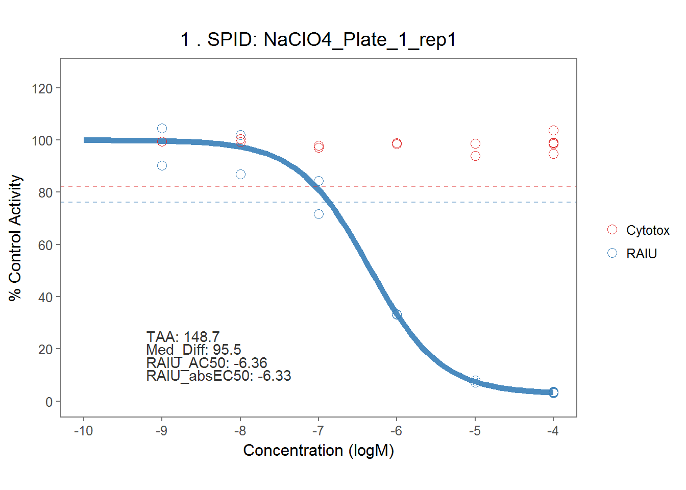

# DCNQ
dt_dcnq <- dt_mc_norm %>% filter(spid == "DCNQ") %>%
    mutate(spid = paste(spid, pid, rep, sep = "_"))
dcnq_md <- fit_curve_tcpl(dt_dcnq,
                                 assay_info = list(prim_assay = "RAIU", toxi_assay = "Cytotox"),
                                 prim_cutoff = 23.78165,
                                 toxi_cutoff = 17.68251)

## Processing 54 samples(spid)....
## DCNQ_Plate_1_rep1 ||DCNQ_Plate_1_rep2 ||DCNQ_Plate_1_rep3 ||DCNQ_Plate_10_rep1 ||DCNQ_Plate_10_rep2 ||DCNQ_Plate_10_rep3 ||DCNQ_Plate_11_rep1 ||DCNQ_Plate_11_rep2 ||DCNQ_Plate_11_rep3 ||DCNQ_Plate_12_rep1 ||DCNQ_Plate_12_rep2 ||DCNQ_Plate_12_rep3 ||DCNQ_Plate_13_rep1 ||DCNQ_Plate_13_rep2 ||DCNQ_Plate_13_rep3 ||DCNQ_Plate_14_rep1 ||DCNQ_Plate_14_rep2 ||DCNQ_Plate_14_rep3 ||DCNQ_Plate_15_rep1 ||DCNQ_Plate_15_rep2 ||DCNQ_Plate_15_rep3 ||DCNQ_Plate_16_rep1 ||DCNQ_Plate_16_rep2 ||DCNQ_Plate_16_rep3 ||DCNQ_Plate_17_rep1 ||DCNQ_Plate_17_rep2 ||DCNQ_Plate_17_rep3 ||DCNQ_Plate_18_rep1 ||DCNQ_Plate_18_rep2 ||DCNQ_Plate_18_rep3 ||DCNQ_Plate_2_rep1 ||DCNQ_Plate_2_rep2 ||DCNQ_Plate_2_rep3 ||DCNQ_Plate_3_rep1 ||DCNQ_Plate_3_rep2 ||DCNQ_Plate_3_rep3 ||DCNQ_Plate_4_rep1 ||DCNQ_Plate_4_rep2 ||DCNQ_Plate_4_rep3 ||DCNQ_Plate_5_rep1 ||DCNQ_Plate_5_rep2 ||DCNQ_Plate_5_rep3 ||DCNQ_Plate_6_rep1 ||DCNQ_Plate_6_rep2 ||DCNQ_Plate_6_rep3 ||DCNQ_Plate_7_rep1 ||DCNQ_Plate_7_rep2 ||DCNQ_Plate_7_rep3 ||DCNQ_Plate_8_rep1 ||DCNQ_Plate_8_rep2 ||DCNQ_Plate_8_rep3 ||DCNQ_Plate_9_rep1 ||DCNQ_Plate_9_rep2 ||DCNQ_Plate_9_rep3 ||
## Curve Fitting Completed!
## Calculation time: 13.5 secs

dcnq_rank <- rank_tcpl(dcnq_md)
dcnq_plots <- plot_tcpl(dcnq_md, dcnq_rank, notation = T)
dcnq_plots[[1]]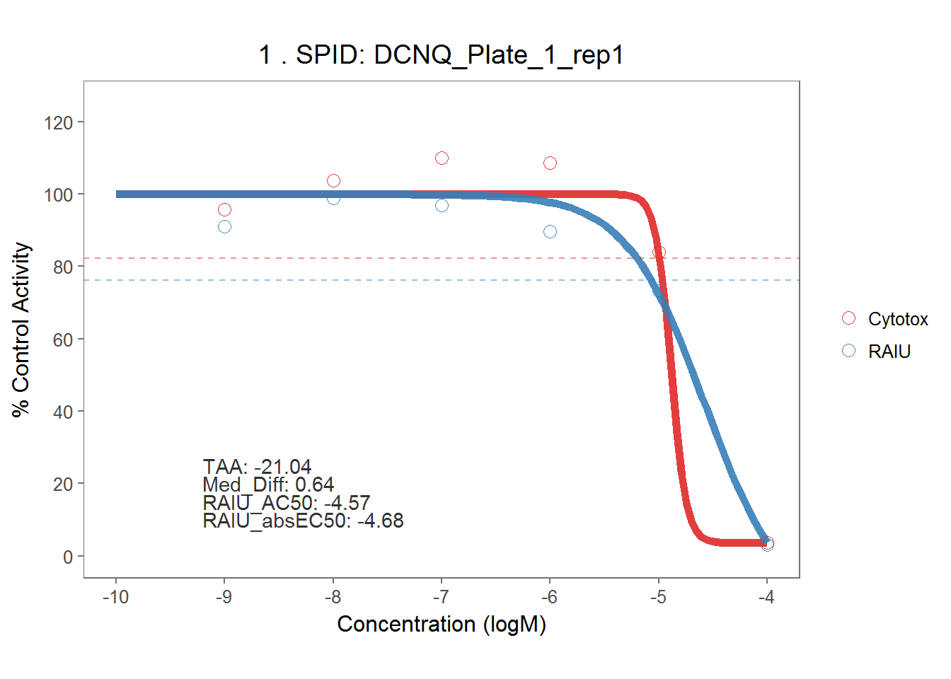

# Export all Sodium Perchlorate and DCNQ plots into one pdf supplemental file
l3 <- append(perchlorate_plots, dcnq_plots)
# save_plot_pdf(l3, "./output plots/perchlorate_dcnq_curves.pdf")

# bind_rows(dt_perchlorate, dt_dcnq) %>% 
#     select(spid, assay, conc, nval_median) %>% 
#     write_csv("./output figure's source data/supplemental_fig.3_data.csv")

5.4.3 Visualize all Multi-Con Controls

Visualize all other controls (DMSO, 2,4-D 100uM, DCNQ 100uM, NaNO3 100uM, NaSCN 100uM) included on each test plate. NaClO4 and DCNQ are plotted using the 100uM concentration wells.

m3 <- dt_mc_norm %>% 
    filter(!wllt %in% c("t")) %>% 
    filter(!(spid %in% c("NaClO4", "DCNQ")))

m4 <- dt_mc_norm %>% 
    filter(spid %in% c("NaClO4", "DCNQ")) %>% 
    filter(conc == 1e-4)

m31 <- bind_rows(m3, m4)

## facet plots of all controls' data points
ggplot(m31, aes(apid, nval_median)) + 
    geom_point(aes(color=apid),alpha=0.7) + 
    facet_grid(spid~assay) +
    scale_y_continuous(limits= c(-20,140), breaks= seq(from=-20, to=140, by=20)) + 
    #scale_x_discrete(breaks=NULL)+
    scale_x_discrete(labels=NULL)+
    ylab("% Control Activity") +
    xlab("Assay Plate ID")+
    ggtitle("Response of controls in all 54 multi-conc assay plates")+
    theme_bw()+
    theme(legend.position = "none",
          plot.title=element_text(hjust=0.5))

##print the control stats table. 
mc_ctrl_sum <- m31 %>% 
    filter(wllt != "t") %>% 
    #mutate(assay= if_else(aeid==1, "Cytotox", "RAIU")) %>%  #add "assay" variable
    mutate(resp=nval_median) %>% 
    group_by(assay, spid) %>% 
    summarize(mean = mean(resp),
              sd = sd(resp),
              min = min(resp),
              max = max(resp),
              CV = sd/mean*100)
knitr::kable(mc_ctrl_sum, digits = 2, caption = "Multi-Conc Control Summary Stats")

Table 5.5: Multi-Conc Control Summary Stats
assay	spid	mean	sd	min	max	CV
Cytotox	2,4-D	99.34	4.21	90.92	113.31	4.24
Cytotox	DCNQ	3.72	0.38	2.62	4.76	10.33
Cytotox	DMSO	100.92	5.41	87.82	123.66	5.36
Cytotox	NaClO4	99.19	4.69	89.12	112.51	4.73
Cytotox	NaNO3	98.95	5.43	88.64	112.92	5.49
Cytotox	NaSCN	104.30	3.98	94.83	117.03	3.81
RAIU	2,4-D	90.86	4.49	76.22	101.30	4.94
RAIU	DCNQ	3.92	3.37	2.58	27.36	85.98
RAIU	DMSO	99.50	8.28	80.77	119.46	8.32
RAIU	NaClO4	3.28	0.38	2.30	4.33	11.47
RAIU	NaNO3	83.08	7.17	69.45	98.80	8.63
RAIU	NaSCN	24.69	2.71	20.47	43.17	10.99

5.5 Test Chemical Dose-response Modeling

The model used here is the Hill model provided in tcpl R package.

\[f(x) = \frac{tp}{1+10^{(ga-x)gw}}\]

Where x is the log concentration, tp is the top asymptote, ga is the AC50 (the log concentration where the modeled activity equals 50% of the top asymptote), and gw is the hill coefficient. The Hill model provided in the tcpl R package constrains the three parameters as following:

1. 0 <= tp <= 1.2 times the maximum response value
1. (minimum log concentration minus 2) <= ga <= (maximum log concentration plus 0.5)
1. 0.3 <= gw <= 8

The modelling is done using a wrapper function fit_curve_tcpl in ToxPlot package, which serves as an convenient interface to use the tcplFit function in the tcpl package, and returns a list object containing all data and modeling results.

mc_model <- fit_curve_tcpl(df = filter(dt_mc_norm, wllt == "t"), 
                           assay_info = list(prim_assay = "RAIU", toxi_assay = "Cytotox"), 
                           prim_cutoff = 23.78165, toxi_cutoff = 17.68251)

## Processing 169 samples(spid)....
## TP0001498A01 ||TP0001498B02 ||TP0001498B05 ||TP0001498B07 ||TP0001498B08 ||TP0001498B09 ||TP0001498B11 ||TP0001498C01 ||TP0001498C03 ||TP0001498C04 ||TP0001501E03 ||TP0001501E05 ||TP0001501E07 ||TP0001501E11 ||TP0001501F01 ||TP0001501F04 ||TP0001501F07 ||TP0001501G02 ||TP0001501G03 ||TP0001501G04 ||TP0001501G09 ||TP0001501G10 ||TP0001501G11 ||TP0001502A01 ||TP0001502B01 ||TP0001502B03 ||TP0001502B04 ||TP0001502B05 ||TP0001502B07 ||TP0001502B10 ||TP0001502C04 ||TP0001502C07 ||TP0001502C09 ||TP0001502C11 ||TP0001502D03 ||TP0001502D04 ||TP0001502D09 ||TP0001502D11 ||TP0001502E01 ||TP0001502E02 ||TP0001502E03 ||TP0001502E04 ||TP0001502E07 ||TP0001502E08 ||TP0001502E10 ||TP0001502F02 ||TP0001502F03 ||TP0001502F04 ||TP0001502F05 ||TP0001502F07 ||TP0001502F09 ||TP0001502F10 ||TP0001502G01 ||TP0001502G02 ||TP0001502G03 ||TP0001502G04 ||TP0001502G07 ||TP0001502G09 ||TP0001502G11 ||TP0001500A01 ||TP0001500B02 ||TP0001500B05 ||TP0001500B07 ||TP0001500B08 ||TP0001500B09 ||TP0001500C04 ||TP0001500C05 ||TP0001500C09 ||TP0001500D03 ||TP0001500D04 ||TP0001500D05 ||TP0001500D07 ||TP0001500D09 ||TP0001500D11 ||TP0001500E01 ||TP0001500E05 ||TP0001500E07 ||TP0001500E08 ||TP0001500E09 ||TP0001500E10 ||TP0001500E11 ||TP0001500F01 ||TP0001500F02 ||TP0001500F03 ||TP0001500F04 ||TP0001500F07 ||TP0001500F09 ||TP0001500F11 ||TP0001500G01 ||TP0001500G02 ||TP0001500G03 ||TP0001500G04 ||TP0001500G05 ||TP0001500G07 ||TP0001500G08 ||TP0001500G09 ||TP0001500G11 ||TP0001498C09 ||TP0001498C10 ||TP0001498C11 ||TP0001498D01 ||TP0001498D02 ||TP0001498D03 ||TP0001498D05 ||TP0001498D07 ||TP0001498D08 ||TP0001498D10 ||TP0001498D11 ||TP0001498E01 ||TP0001498E04 ||TP0001498E08 ||TP0001498E11 ||TP0001498F01 ||TP0001498F03 ||TP0001498F05 ||TP0001498F07 ||TP0001498G01 ||TP0001498G02 ||TP0001498G03 ||TP0001498G05 ||TP0001498G08 ||TP0001498G09 ||TP0001498H12 ||TP0001499A01 ||TP0001499B01 ||TP0001499B03 ||TP0001499B05 ||TP0001499B07 ||TP0001499B11 ||TP0001499C01 ||TP0001499C07 ||TP0001499C08 ||TP0001499C09 ||TP0001499D01 ||TP0001499D02 ||TP0001499D08 ||TP0001499E01 ||TP0001499E02 ||TP0001499E03 ||TP0001499E09 ||TP0001499E10 ||TP0001499E11 ||TP0001499F01 ||TP0001499F10 ||TP0001499G01 ||TP0001499G02 ||TP0001499G03 ||TP0001499G10 ||TP0001499G11 ||TP0001501A01 ||TP0001501B01 ||TP0001501B05 ||TP0001501B08 ||TP0001501B10 ||TP0001501B11 ||TP0001501C01 ||TP0001501C02 ||TP0001501C03 ||TP0001501C04 ||TP0001501C09 ||TP0001501C11 ||TP0001501D01 ||TP0001501D02 ||TP0001501D03 ||TP0001501D04 ||TP0001501D05 ||TP0001501D10 ||TP0001501E01 ||TP0001501E02 ||
## Curve Fitting Completed!
## Calculation time: 37.7 secs