4 Single-Conc Results Analysis

rm(list=ls())
library(plotly)
library(ggthemes)
library(stringr)
library(readxl)
library(grid)
library(gridExtra)
library(devtools)
# load_all("./toxplot first pub ver")
load_all("./toxplot")
library(tidyverse)
# session_info()

4.1 Define basic assay info

  #define the names of the primary and toxicity assay.
  #names should match what's provided in the <assay> column of the input dataframe
assay_info <- list(
  prim_assay = "RAIU",
  toxi_assay = "Cytotox"
)

4.2 Data Import

dt_sc <- read_csv("./input data files/NIS_ph1_v2_sc_lvl0_for_tcpl.csv")

4.3 Normalization

Each sample well is normalized as percentage of the DMSO median on each plate.

dt_sc_norm <- toxplot::normalize_per_plate(dt_sc, nctrl = "DMSO")

4.4 Threshold of Significance

Now calculating 3bMAD and 3sigma value for the DMSO control in the single concentration assay as a whole.

sig_cutoff_sc <- dt_sc_norm %>% 
    filter(spid == "DMSO") %>% 
    summarize(bMAD = mad(nval_median, na.rm=TRUE),
              three_bMAD = 3*mad(nval_median, na.rm=TRUE)) 
knitr::kable(sig_cutoff_sc, digits = 2) 

bMAD	three_bMAD
6.83	20.5

4.5 QC of Single-conc assay

Assay quality control measures were calculated by each 96-well plate.

To assesss the quality of assay for each 96 well plate, the following metrics were used:

• CV of DMSO controls
• Z’ score

The negative control DMSO wells’ raw readings were used to calculate mean, standard deviation and CV for each plate.

Z’ factor is calculated as follows: \[Z'=1-\frac{3\sigma_{positive\ control} + 3\sigma_{DMSO\ control}}{|\mu_{positive\ control} - \mu_{DMSO\ control}|}\]

Note that in Z’ calculation, because we only had one well of cytotox positive control, therefore sigma wasn’t calculatable. Hence the Z’ calculated for cytotox is unusable.

qc_sc <- qc_per_plate(dt_sc_norm, assay_info, resp = "nval_median")

qplot(unique_id, CV_DMSO, data = qc_sc$qc, color = assay) +
    ggtitle("CV of DMSO in Single-Con Assay") +
    xlab("Assay Plate ID") +
    scale_x_discrete(labels = NULL) +
    theme_bw()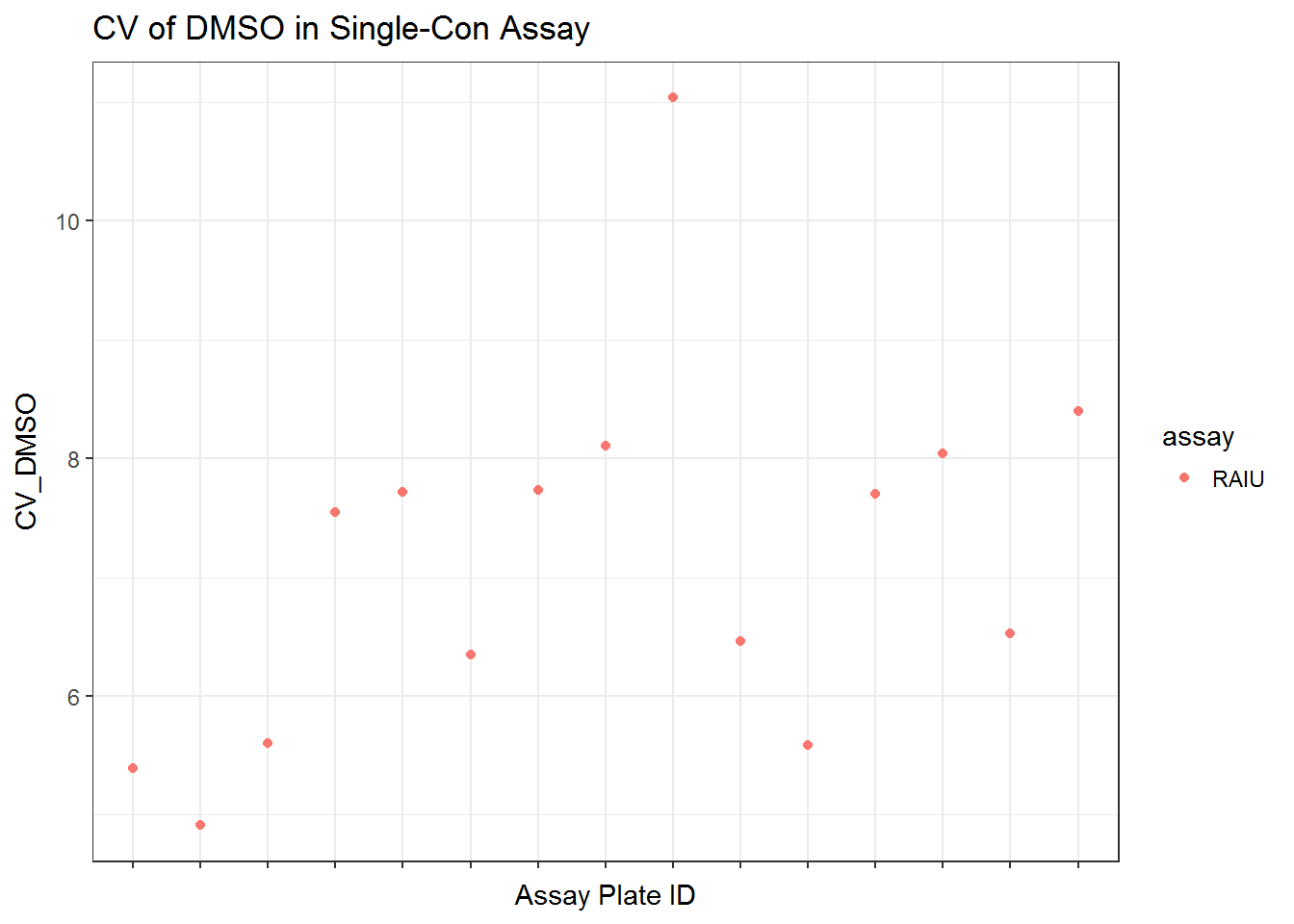

qplot(unique_id, Z_prime, data = qc_sc$qc, color = assay) +
    ggtitle("Z' in Single-Con Assay") +
    xlab("Assay Plate ID") +
    scale_x_discrete(labels = NULL) +
    theme_bw()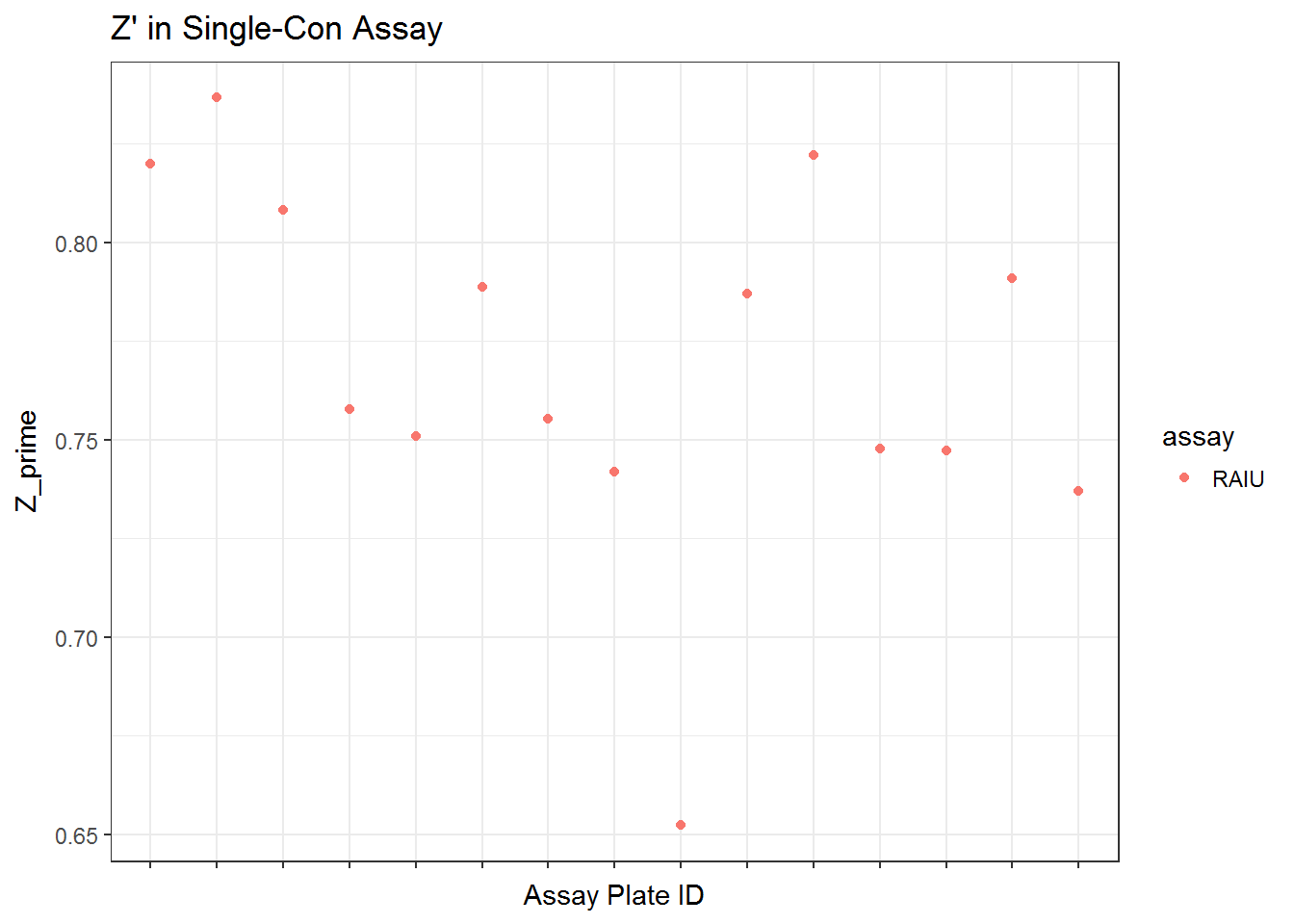

4.6 QC Summary of Single-Con assay

library(psych)
qc_sc_t <- qc_sc$qc %>%
    dplyr::select(CV_DMSO, Z_prime) %>%
    describe
knitr::kable(qc_sc_t, digits = 2,  caption = "Summary Single-Con Assay QC Metrics")

Table 4.1: Summary Single-Con Assay QC Metrics

	vars	n	mean	sd	median	trimmed	mad	min	max	range	skew	kurtosis	se
apid*	1	15	NaN	NA	NA	NaN	NA	Inf	-Inf	-Inf	NA	NA	NA
CV_DMSO	2	15	7.14	1.56	7.55	7.01	1.52	4.91	11.04	6.13	0.68	0.19	0.40
Z_prime	3	15	0.77	0.05	0.76	0.77	0.04	0.65	0.84	0.18	-0.72	0.40	0.01

All single-con QC metrics in a table

knitr::kable(dplyr::select(qc_sc$qc, apid, CV_DMSO, Z_prime),
             digits = 2,
             col.names = c("Plate", "CV of DMSO", "Z'"),
             caption = "QC metrics in Single-Conc Screening")

Table 4.2: QC metrics in Single-Conc Screening

Plate	CV of DMSO	Z’
TP0001498_rep1	5.40	0.82
TP0001498_rep2	4.91	0.84
TP0001498_rep3	5.61	0.81
TP0001499_rep1	7.55	0.76
TP0001499_rep2	7.72	0.75
TP0001499_rep3	6.35	0.79
TP0001500_rep1	7.74	0.76
TP0001500_rep2	8.11	0.74
TP0001500_rep3	11.04	0.65
TP0001501_rep1	6.46	0.79
TP0001501_rep2	5.59	0.82
TP0001501_rep3	7.70	0.75
TP0001502_rep1	8.04	0.75
TP0001502_rep2	6.53	0.79
TP0001502_rep3	8.40	0.74

4.6.1 Single-Con Positive Control QC

## model single-con controls on each plate
sc_pos_raiu <- dt_sc_norm %>% 
    filter(spid == "NaClO4") %>% 
    mutate(spid = paste(spid, apid)) # change spid to distinguish NaClO4 on each plate. 

sc_raiu_pos_md <- toxplot::fit_curve_tcpl(sc_pos_raiu, assay_info = list(prim_assay = "RAIU", toxi_assay = NULL))

## Processing 15 samples(spid)....
## NaClO4 TP0001498_rep1 ||NaClO4 TP0001498_rep2 ||NaClO4 TP0001498_rep3 ||NaClO4 TP0001499_rep1 ||NaClO4 TP0001499_rep2 ||NaClO4 TP0001499_rep3 ||NaClO4 TP0001500_rep1 ||NaClO4 TP0001500_rep2 ||NaClO4 TP0001500_rep3 ||NaClO4 TP0001501_rep1 ||NaClO4 TP0001501_rep2 ||NaClO4 TP0001501_rep3 ||NaClO4 TP0001502_rep1 ||NaClO4 TP0001502_rep2 ||NaClO4 TP0001502_rep3 ||
## Curve Fitting Completed!
## Calculation time: 2.8 secs

sc_raiu_pos_sum <- toxplot::summary_tcpl(sc_raiu_pos_md)

##plot AC50 for pos controls together
st <- sc_raiu_pos_sum %>% 
    dplyr::select(AC50_prim, absEC50_prim, spid) %>% 
    rename(AC50 = AC50_prim, absEC50 = absEC50_prim) %>% 
    gather(key=Metric, value= value, AC50, absEC50)

ggplot(st, aes(spid, value)) +
    geom_point(aes(color=Metric), alpha=0.8, size=3)+
    #facet_grid(Metric~., scale="free")+
    scale_x_discrete(labels=NULL)+
    ggtitle("AC50 & absEC50 of Positive Control(NaClO4) in Single-Con Assay")+
    xlab("Assay Plate ID") +
    ylab("Concentration (logM)") +
    theme(plot.title = element_text(hjust=0.5)) +
    theme_bw()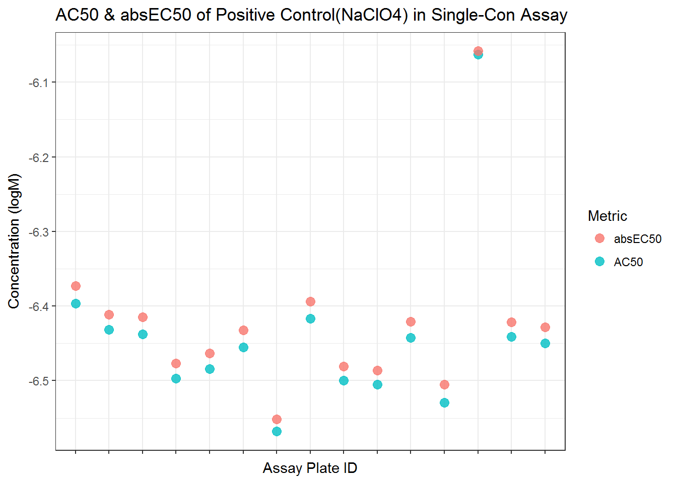 

    #theme(legend.position = "none") 

#summary
library(psych)
sc_pos_sum_raiu <- sc_raiu_pos_sum %>%
    dplyr::select(AC50_prim, absEC50_prim) %>% 
    rename(AC50=AC50_prim, absEC50 = absEC50_prim) %>% 
    describe
knitr::kable(sc_pos_sum_raiu, digits = 2,  caption="Summary of single-con RAIU positive control IC50s")

Table 4.3: Summary of single-con RAIU positive control IC50s

	vars	n	mean	sd	median	trimmed	mad	min	max	range	skew	kurtosis	se
AC50	1	15	-6.44	0.11	-6.45	-6.46	0.05	-6.57	-6.06	0.51	2.28	5.19	0.03
absEC50	2	15	-6.42	0.11	-6.43	-6.44	0.05	-6.55	-6.06	0.49	2.18	4.85	0.03

4.6.2 Single-Con Controls

#only take the NaClO4 wells at 1E-4M
s1 <- dt_sc_norm %>% filter(wllt!="t", spid!="NaClO4")
s2 <- dt_sc_norm %>% filter(spid=="NaClO4", conc== 1E-4)
s3 <- bind_rows(s1, s2)

sc_ctrl_sum <- s3 %>% 
    filter(wllt !="t") %>% 
    mutate(resp=nval_median) %>% 
    #rename("NaClO4(1E-4M)F"=NaClO4) %>% 
    group_by(spid) %>% 
    summarize(mean = mean(resp),
              sd = sd(resp),
              min = min(resp),
              max = max(resp),
              CV = sd/mean*100)
knitr::kable(sc_ctrl_sum, digits =2, caption="Single-Con control summary stats")

Table 4.4: Single-Con control summary stats

spid	mean	sd	min	max	CV
2,4-D	92.41	4.24	83.91	100.71	4.59
DMSO	100.63	7.11	71.69	116.19	7.06
NaClO4	2.85	0.36	2.08	3.84	12.60
NaNO3	81.25	7.56	63.47	93.21	9.31
NaSCN	20.64	1.12	18.56	23.05	5.41

# plot all sc controls
ggplot(filter(s3, wllt !="t"), aes(apid, nval_median)) + 
    geom_point(aes(color=apid),alpha=0.6) + 
    facet_grid(spid~.) +
    scale_y_continuous(limits= c(-20,140), breaks= seq(from=-20, to=140, by=20)) + 
    #scale_x_discrete(breaks=NULL)+
    scale_x_discrete(labels=NULL)+
    ylab("Normalized Response") +
    xlab("Assay Plate ID")+
    ggtitle("Response of controls in 15 Single-Conc assay plates")+
    theme_bw()+
    theme(legend.position = "none") +
    theme(plot.title=element_text(hjust=0.5))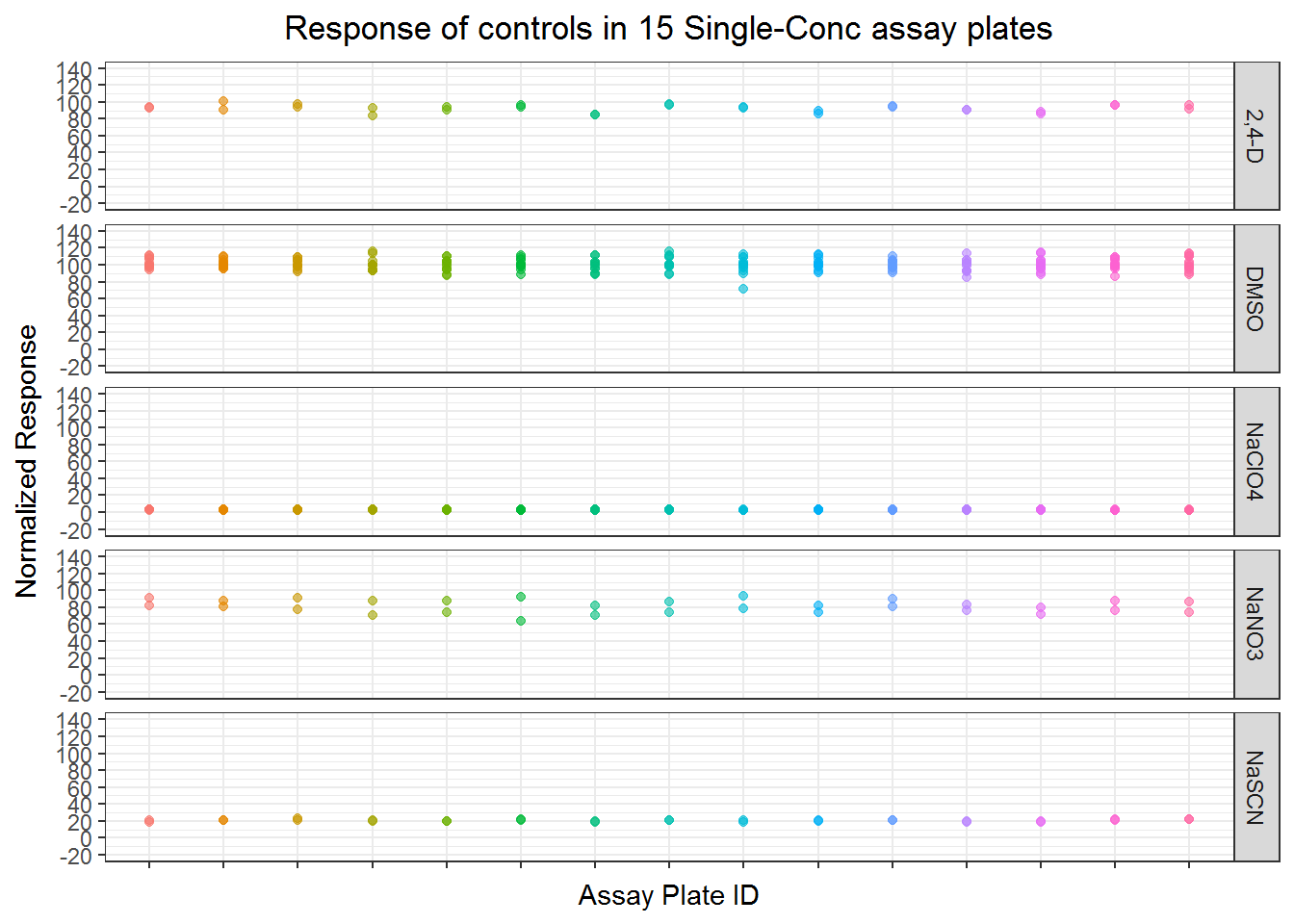

4.7 Visualize the single concentration data

A total of 310 chemical samples was tested in the single-con and 169 were further tested in multi-concentration.
The plot below showed the median, max, and min value for each tested chemical, and coloring shows which chemical were carried on to the multi-con assay. Because the assay has 3 replicates, so all three replicate’s data are actually plotted in this figure.

#calculate median, max and min value
sc_median <- dt_sc_norm %>% ungroup() %>% filter(str_detect(dt_sc_norm$spid, "^TP*")) %>% 
    mutate(welltype = "sample") %>%
    group_by(pid, spid) %>%
    summarize(
        median = median(nval_median),
        up_range = max(nval_median),
        lo_range = min(nval_median),
        range = max(nval_median) - min(nval_median)
    ) %>%
    ungroup() %>%
    mutate(mc_test = ifelse(median < 80, "Yes", "No")) %>%
    arrange(median)
#saveRDS(sc_median, "../../NIS project Phase II/Phase 2 data analysis/ph1_single.rds")
##Plot single con median+range plot. 
library(RColorBrewer)

fig2 <- ggplot(sc_median, aes(x=reorder(spid, -median), y=median, color=mc_test)) +
    geom_point(size=1.5, alpha=0.6) +
    geom_errorbar(aes(ymax=up_range, ymin=lo_range), alpha=0.8, size = 0.5) +
    xlab("Chemicals, ordered by increasing iodide uptake inhibition") +
    ylab("Iodide Uptake (% of control)")+scale_x_discrete(breaks=NULL) +
    #ggtitle("Median and Response of Test Chemicals")+
    geom_hline(yintercept = 80, linetype="dashed", color="violetred1") +
    geom_hline(yintercept = 100, alpha=0.8) +
    geom_text(data = NULL, x = 270, y = 103, label = "DMSO Control", color = "grey30")+
    geom_text(data = NULL, x = 270, y = 83, label = "20% Inhibition", color = "grey30")+
    scale_y_continuous(breaks = seq(from = 0, to =100, by=20))+
    scale_color_brewer(palette="Set1", name= "Multi-Conc Assay", labels= c("No", "Yes")) +
    theme_few(base_size = 12) +
    theme(legend.position = c(0.15, 0.1), legend.background = element_blank())
fig2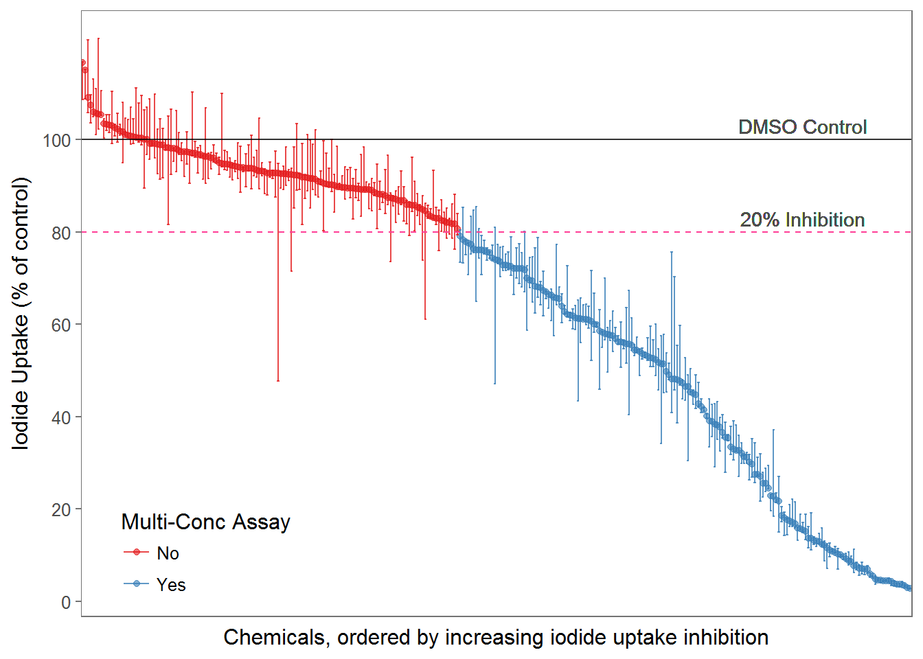

#ggsave("./output plots/fig2.tiff", fig2, dpi = 900, width = 7, height = 5, compression = "lzw")