7 ToxCast Internal Replicates

7.0.1 Single-con internal Replicate performance

ToxCast Ph1_v2 library included internal replicates. They are the same chemical but under different sample id, therefore tested blindly with each sample repliated three times. .

There are 12 chemicals been repeated, showed in the following table

name_code <- spid_chnm_table %>% dplyr::select(spid, casn, chnm)
#check which chemical is repeated in toxcast ph1_v2 library
chnm_freq <- data.frame(table(name_code$chnm)) %>% arrange(desc(Freq))
internal_rep <- head(chnm_freq, 12) 
knitr::kable(internal_rep)

Var1	Freq
2,4-Dichlorophenoxyacetic acid	3
Azoxystrobin	3
Bisphenol A	3
Mancozeb	3
Triclosan	3
Allethrin	2
Bensulide	2
Clorophene	2
Dibutyl phthalate	2
Oryzalin	2
PFOS	2
Triadimenol	2

#spid_chnm_table %>% filter(chnm %in% internal_rep$Var1) %>% View()

##add chnm to sc data
sc_unblind <- left_join(dt_sc_norm, name_code, by= "spid")
## get sc data for interval replicates
sc_rep <- sc_unblind %>% dplyr::filter(chnm %in% internal_rep$Var1)
sc_rep$chnm <- str_replace(sc_rep$chnm, "2,4-Dichlorophenoxyacetic acid", "2,4-D")

sc_rep %>%
    dplyr::select(chnm, pid, nval_median) %>%
    write_csv("./output figure's source data/Fig.3a.data.csv")

library(RColorBrewer)
ir1 <- ggplot(sc_rep, aes(x=reorder(chnm, -nval_median), y=nval_median) ) +
    geom_point(size=2, alpha = 0.8, aes(shape=pid, color=chnm), position = position_jitter(width=0.3)) +
    xlab("") +
    ylab("Iodide Uptake (% of Control)")+
    geom_hline(yintercept = 80, linetype="dashed", color="violetred1") +
    geom_hline(yintercept = 100, alpha=0.8) +
    scale_y_continuous(breaks = seq(from = 0, to =100, by=20))+
    theme_bw(base_size = 12) +
    theme(axis.text.x  = element_text(angle=35, vjust=1, hjust=1),
          #axis.text.y = element_text(size = 12))+
          axis.title = element_text(size = rel(0.8)))+
    #theme(plot.margin = NULL) +
    theme(legend.position="none") 
ir1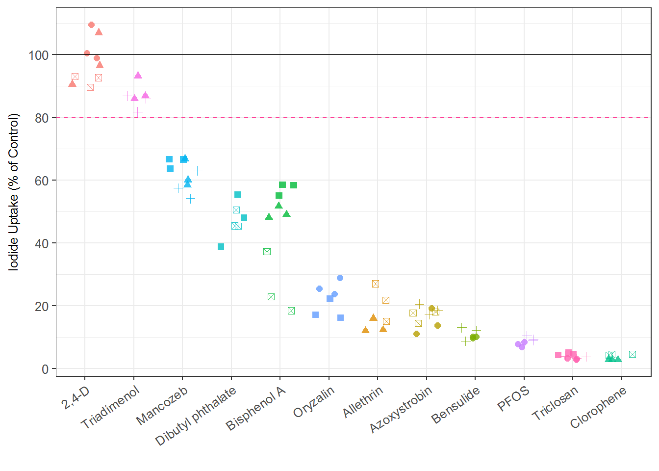

# dev.off()

7.0.2 Multi-con internal controls replication performance

##add chnm to mc data
mc_unblind <- left_join(dt_mc_norm, name_code, by= c("spid"="spid"))

##gettting reps's metrics
mc_rep_sum <- 
    sum_tbl %>% filter(chnm %in% internal_rep$Var1) 

## getting range of ac50s
mc_rep_sum %>% 
    filter(!is.na(AC50_prim)) %>% 
    group_by(chnm) %>% 
    summarize(min = min(AC50_prim), 
              max= max(AC50_prim), 
              range = min - max) %>% 
    arrange(desc(range)) %>% 
    knitr::kable(digits = 2, caption = "Range of AC50 for internal replicates")

Table 7.1: Range of AC50 for internal replicates

chnm	min	max	range
Dibutyl phthalate	-4.54	-4.53	-0.02
PFOS	-4.75	-4.72	-0.02
Oryzalin	-4.38	-4.35	-0.03
Bisphenol A	-4.36	-4.30	-0.06
Bensulide	-4.42	-4.31	-0.11
Triclosan	-5.06	-4.92	-0.14
Mancozeb	-4.92	-4.75	-0.17
Azoxystrobin	-4.58	-4.39	-0.19
Clorophene	-4.87	-4.64	-0.22
Allethrin	-4.52	-4.27	-0.24

# mc_rep_sum %>%
#     dplyr::select(chnm, AC50_prim) %>%
#     write_csv("./output figure's source data/Fig.3b.data.csv")

# write_csv("./output data files/internal_rep_ac50_range.csv")

##plot all points of ac50

ir2 <- ggplot(mc_rep_sum, aes(x=reorder(chnm, AC50_prim), y=AC50_prim) ) +
    geom_point(size = 2, alpha = 0.6, shape = 16) +
    xlab("") +
    ylab("AC50 (logM)")+
    ylim(-6, -4)+
    theme_bw(base_size = 12) +
    theme(axis.text.x  = element_text(angle=30, vjust=1, hjust=1),
          #axis.text.y = element_text(size = 5),
          legend.position = "none",
          axis.title = element_text(size = rel(0.8))
          #plot.margin = NULL
          )


ir2

## Warning: Removed 1 rows containing missing values (geom_point).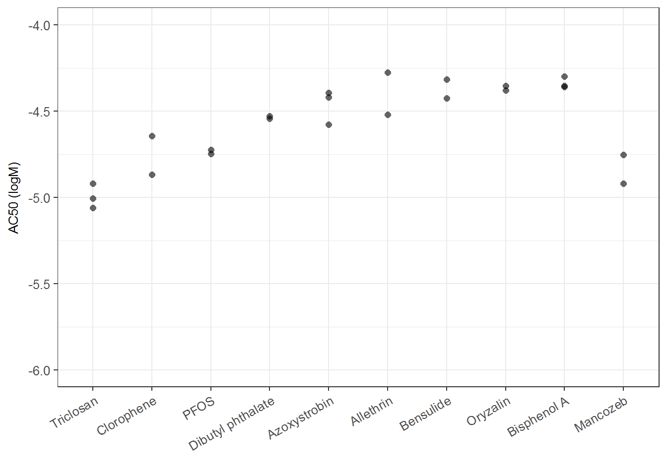

# dev.off()


ir <- arrangeGrob(ir1, ir2)

## Warning: Removed 1 rows containing missing values (geom_point).

# ggsave("./output plots/Fig3.png", ir, dpi=900, width=5, height=6)